

Data processing is the most exciting part of any survey, and bathymetric surveys are no exception. Often, data processing looks overcomplicated, especially if you are trying to use professional software—just because these software packages have dozens of options for almost all possible cases. But if you are working using the same set of equipment and in more or less the same conditions, the processing workflow can be pretty simple and repeatable.
The procedure demonstrated below is for the most straightforward case—the data was collected when the GNSS receiver used for data geotagging was in RTK mode, meaning that we already have precise coordinates and antenna elevation in the data. If we use a PPK receiver or water surface (tide level) data, the workflow will be slightly different, but in general, it will be the same.
Data & software
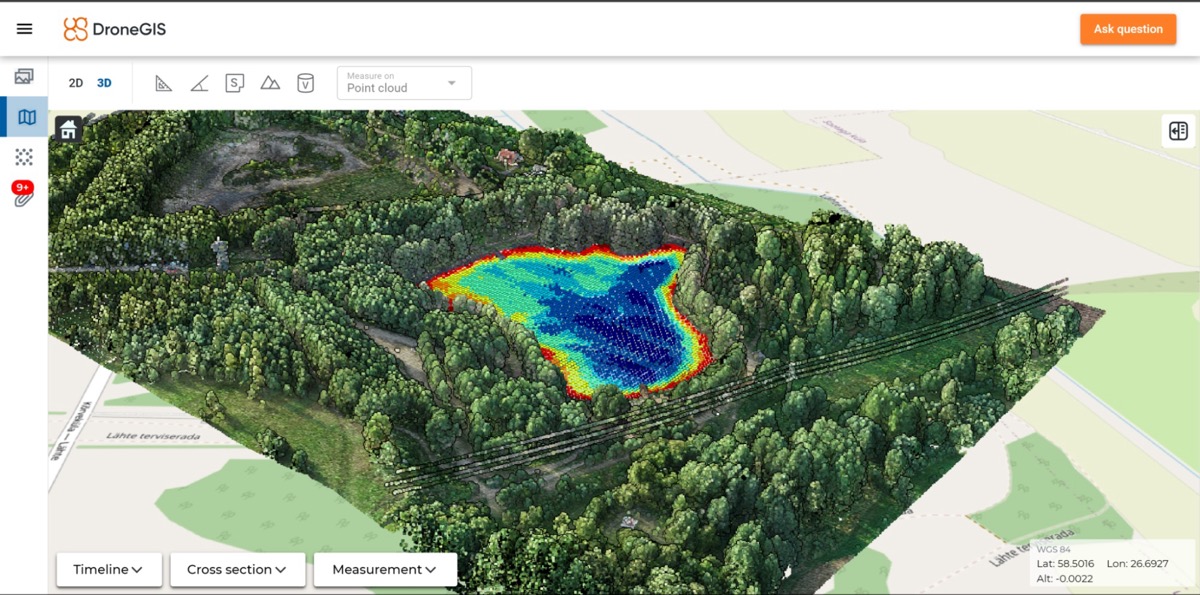
Here I use data gathered in a lake near Tartu, Estonia, in 2022. Data was gathered using Echologger ECT D052 dual-frequency echo sounder mounted on the drone.
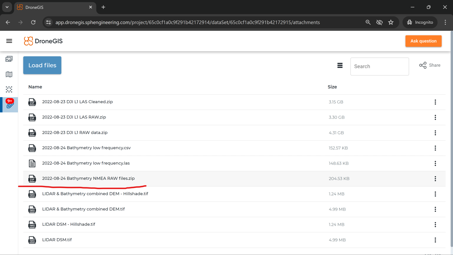
Click Clip icon to navigate to the Attachments and download the archive with NMEA raw data:
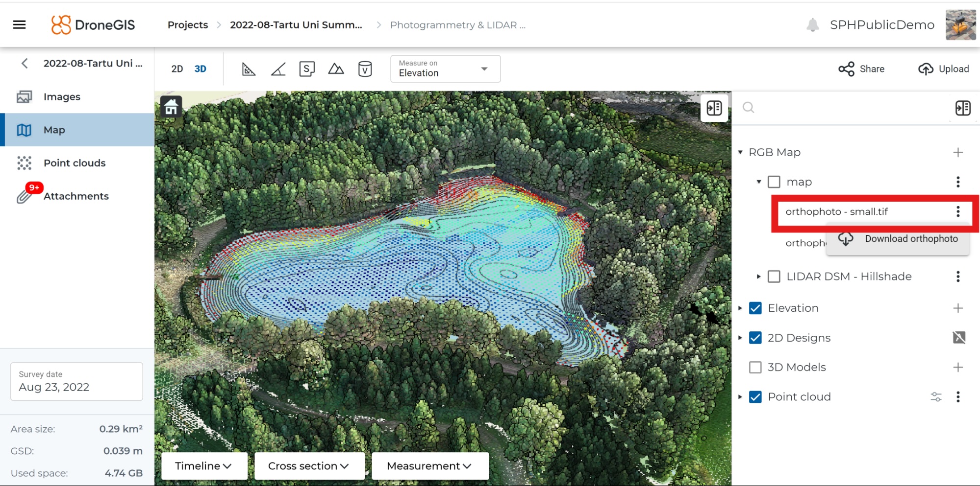
Optionally, you can also download an orthophoto map to use as background in Hydromagic (please note that you need a "small" version - Hydromagic can't handle big images):
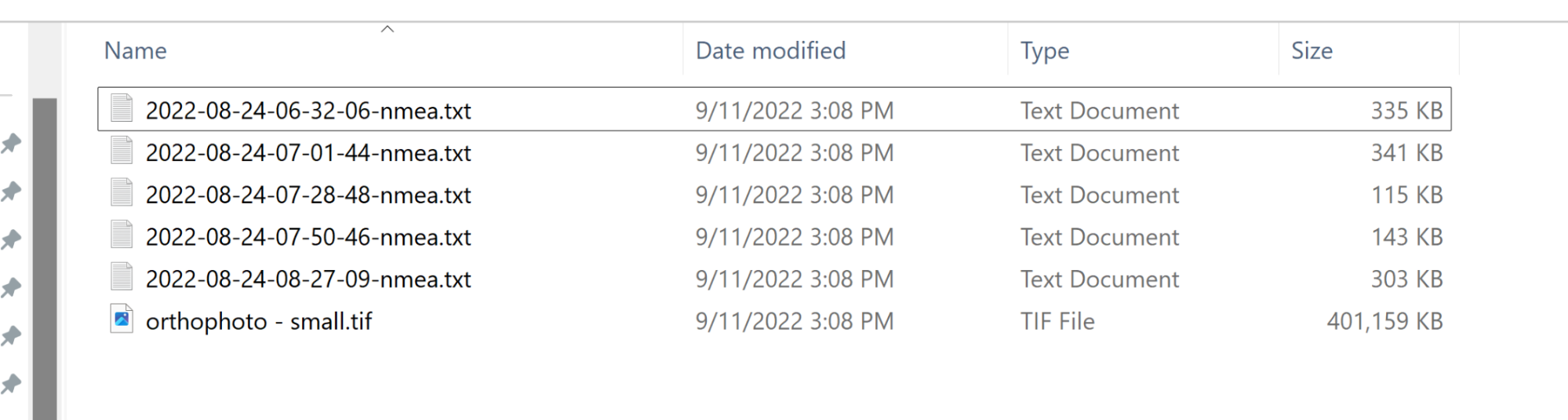
Copy and unpack files to some directory; in my case, it will be C:\Prj\Tartu - we will need 5x files with names like XXX-nmea.txt (data from echo sounder) and orthophoto.
Software
- In this article, I use the latest version (at the date of writing) of Hydromagic (Build 11.0.64.307.)
- Download the trial version: www.eye4software.com/download
Time to open Hydromagic, and let's begin!
Data Import
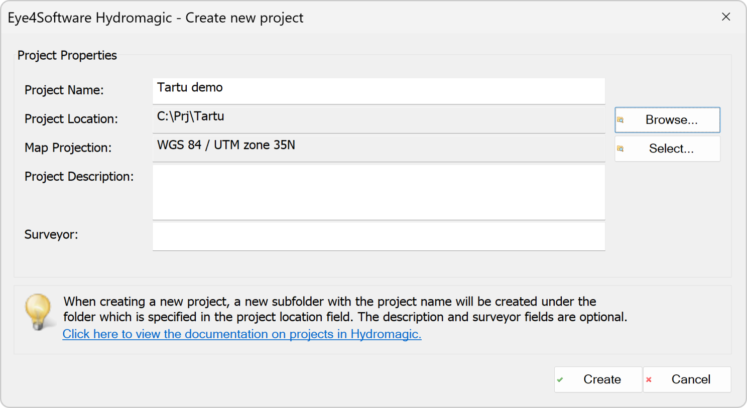
1. Start Hydromagic, and click New Project. Enter the name of the project, select the folder where the project files will reside, and select projection. In most cases, your customer will require output deliverables in some projected coordinate system, here, I selected "WGS 84 / UTM zone 35N". Click Create.
Note: here, I had to select UTM as the projected coordinate system as the orthophoto I want to use uses "WGS 84 / UTM zone 35N." Unfortunately, Hydromagic can't do raster data reprojection. If you need to use maps in a projection different from your required project projection, you can use any GIS for reprojection. I personally use QGIS.
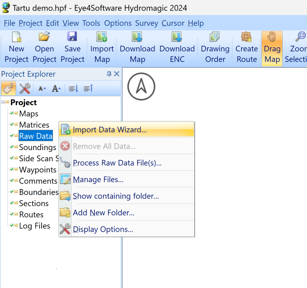
2. Right-click Raw Data in Project Explorer and select Import Data Wizard.
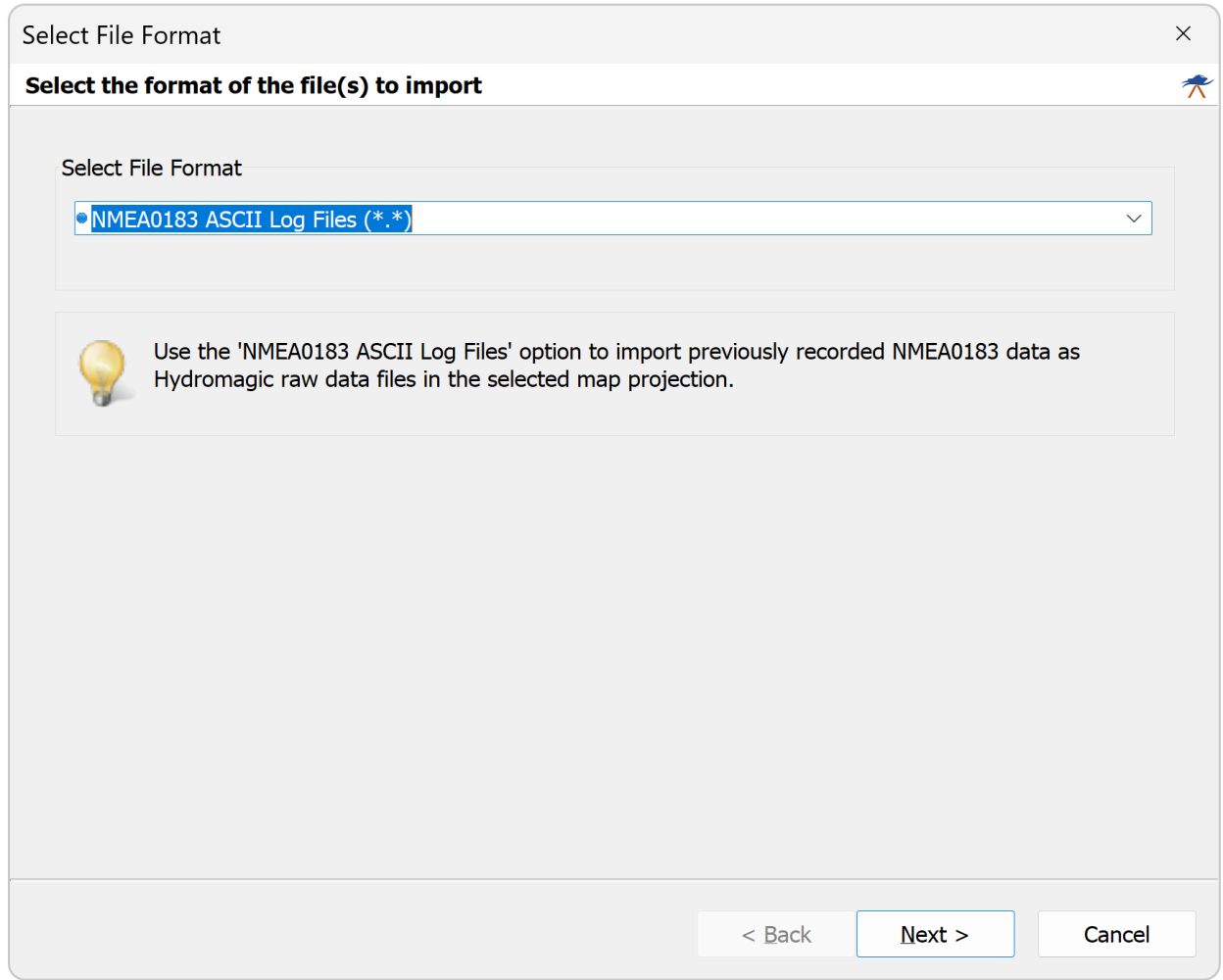
3. Select NMEA0183 ASCII Log Files and click Next.
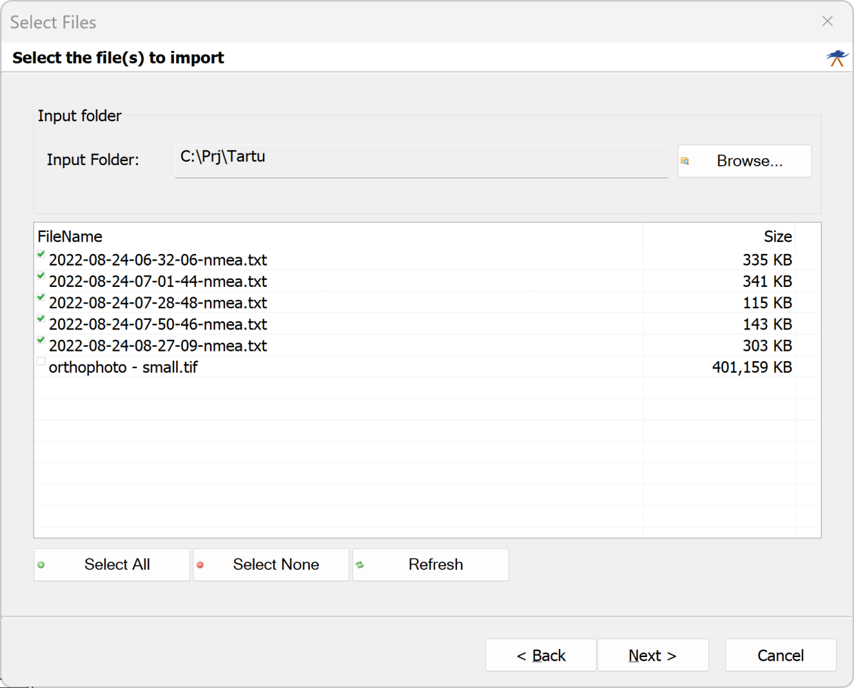
4. Click Browse, select the folder with our NMEA0183 data files, select (set marks) all our data files, and click Next.
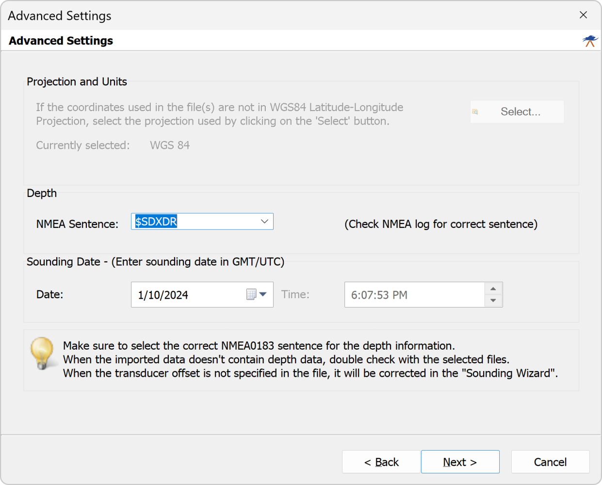
5. Select $SDXDR in the NMEA Sentence drop-down list and click Next and Finish at the next step.
SDXDR sentence stores both high and low frequency readings from the echo sounder.
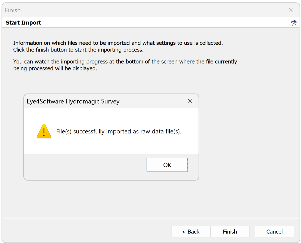
6. Click OK.
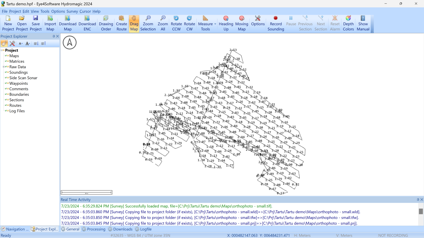
7. We should see the track of raw data below:
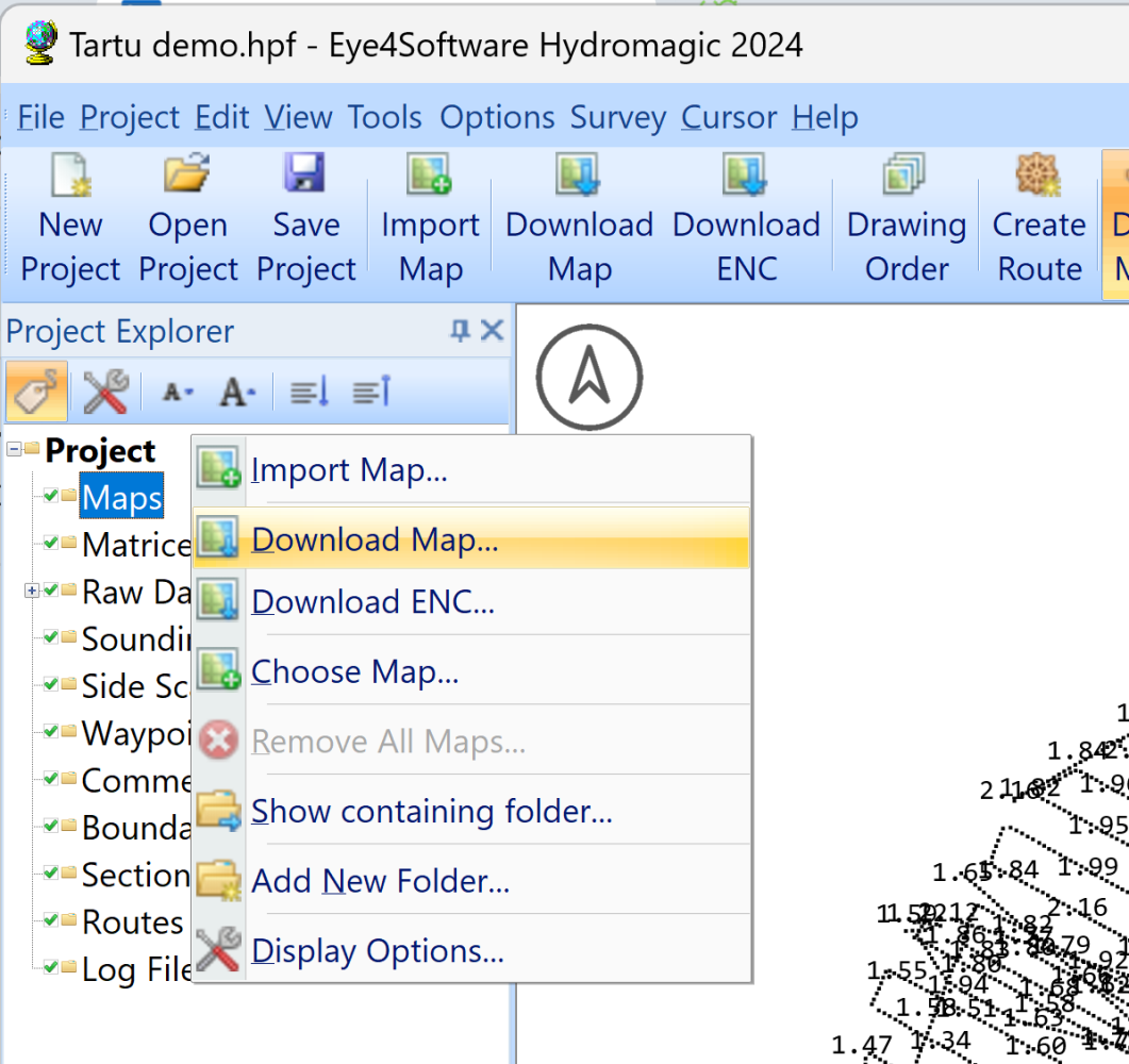
8. Righ-click Maps in Project Explorer and select Download Map
9. Select your favorite map source and click Calculate.
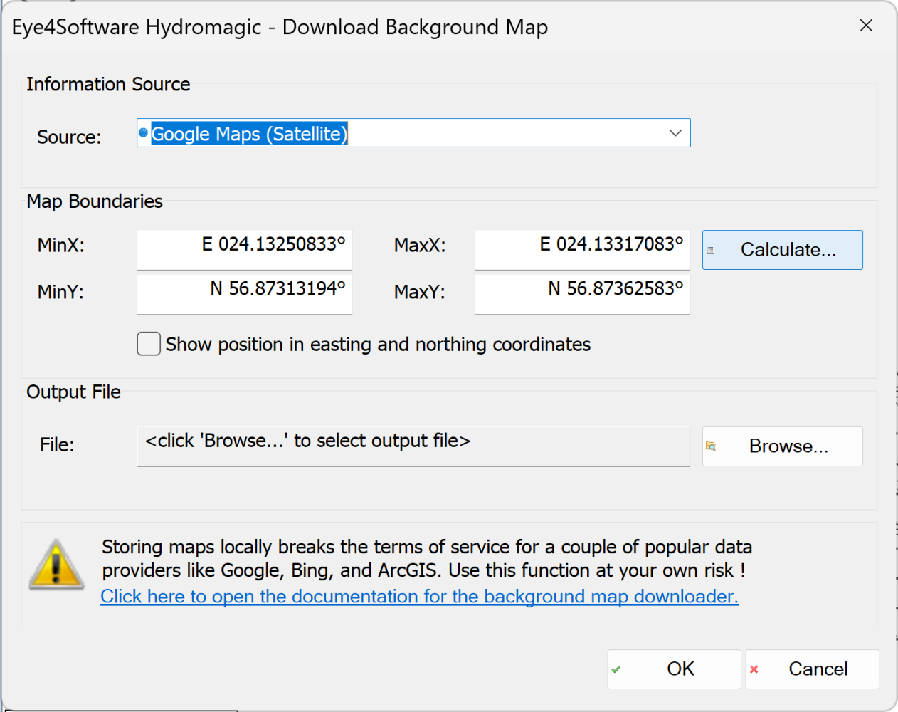
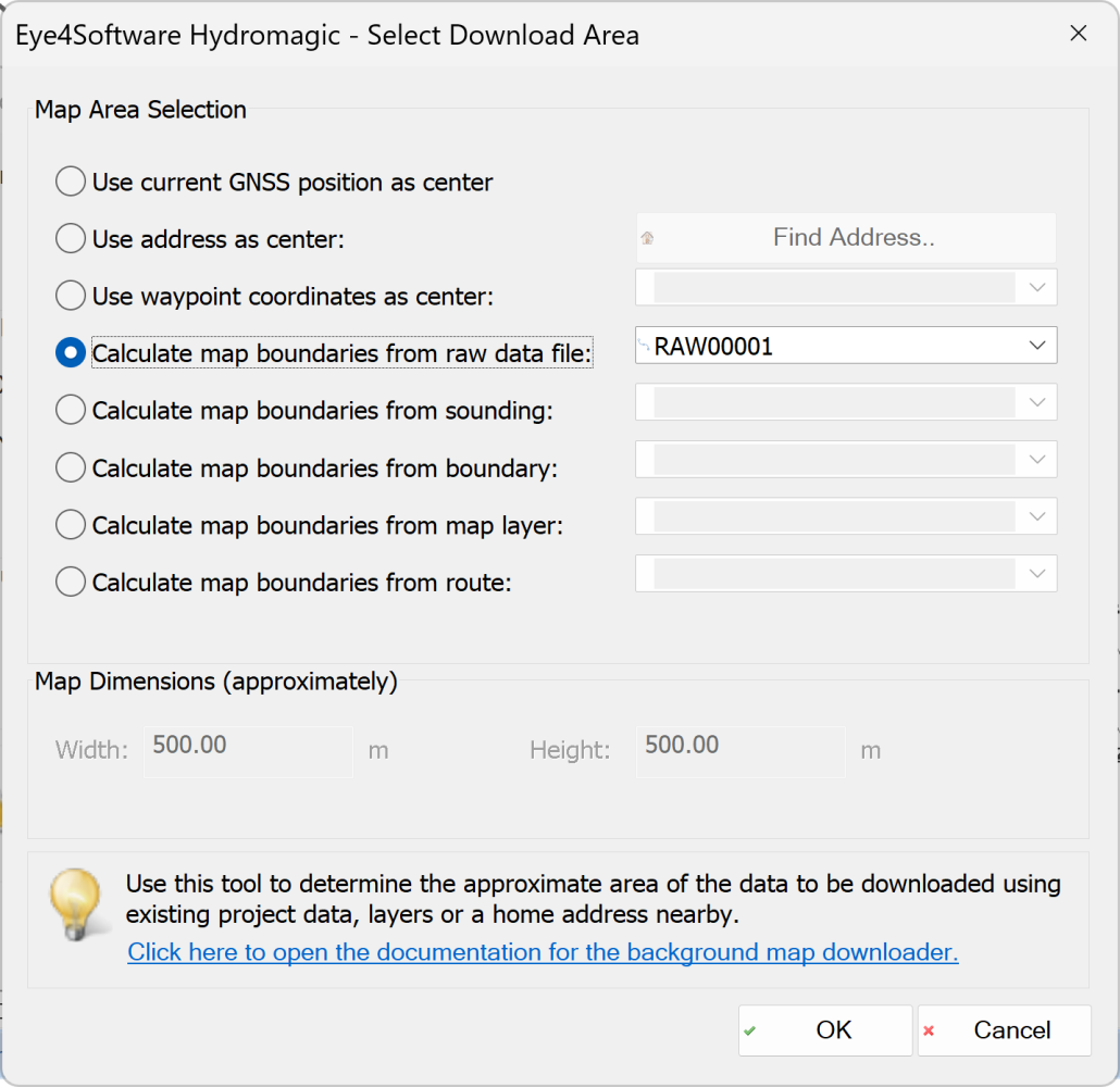
10. Select "Calculate map boundaries from raw data file" and click OK
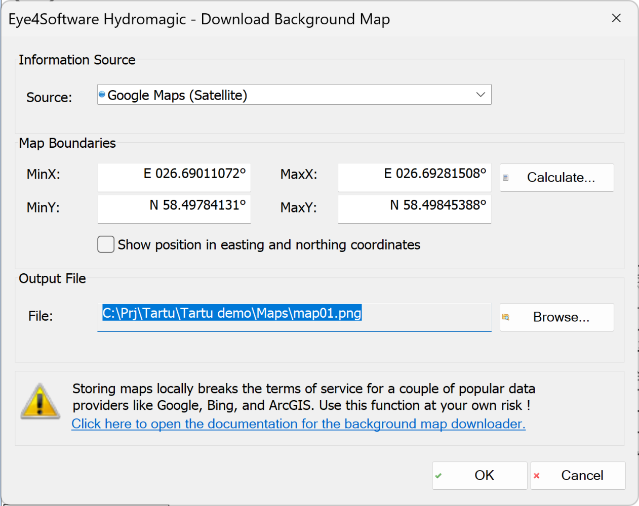
11. Click Browse and select folder and file name for the map. Click OK.
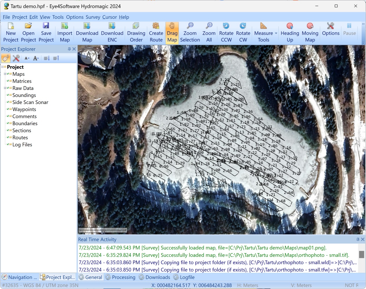
12. Enjoy the map in background. Brrrr, winter...
Real value of this operation - you can see that your data is in right place.
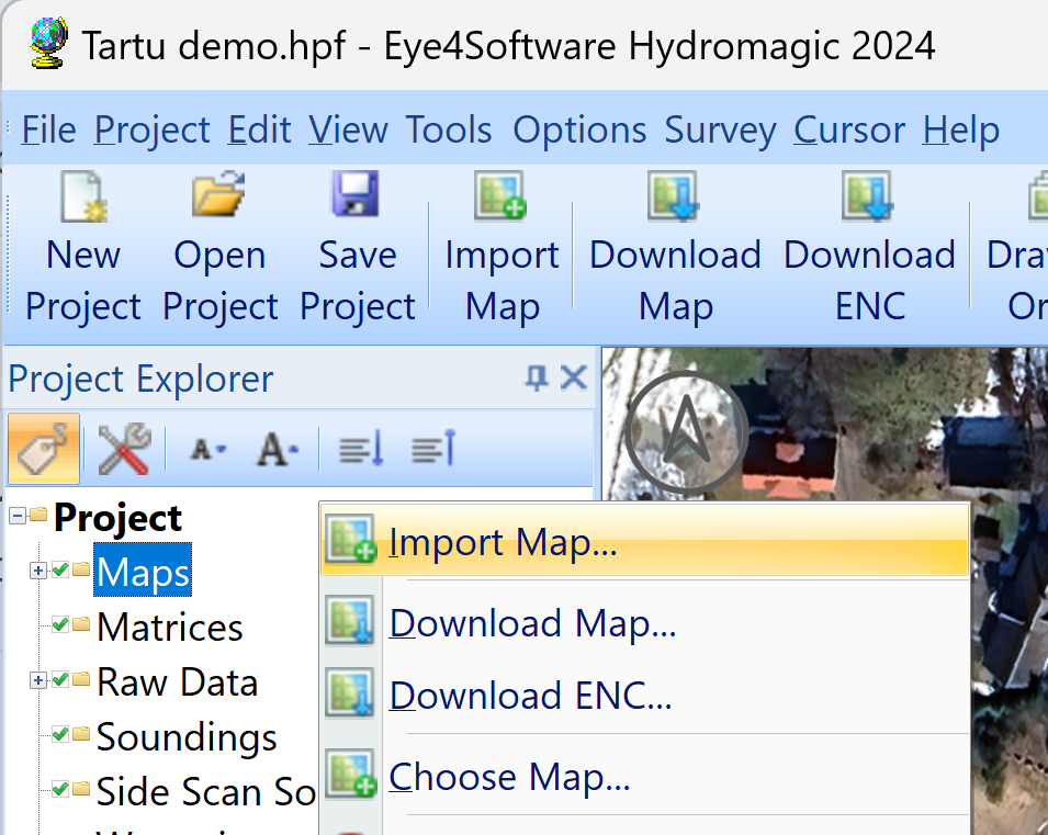
13. If you downloaded our hi-resolution orthophoto, right-click Maps one more time and select Import Map
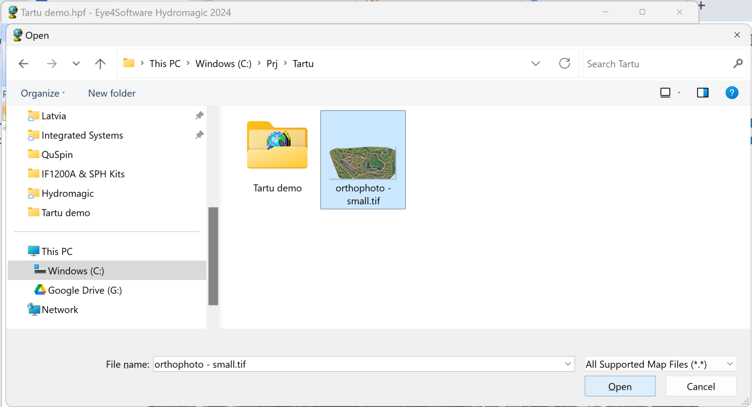
- Select "orthophoto - small.tif" file and click Open
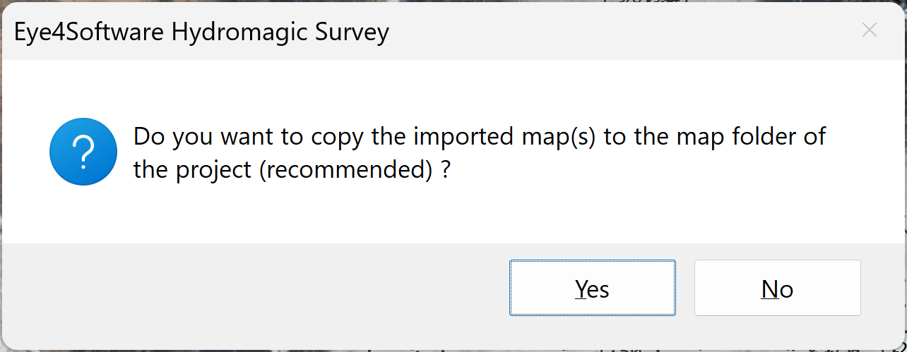
15. Right answer is Yes!
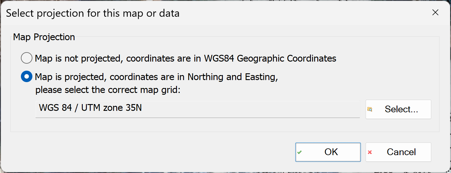
16. Select "Map is projected..." and "WGS 84 / UTM zone 53N". Click OK
17. We can now see two overlapping satellite maps and the same raw data track.
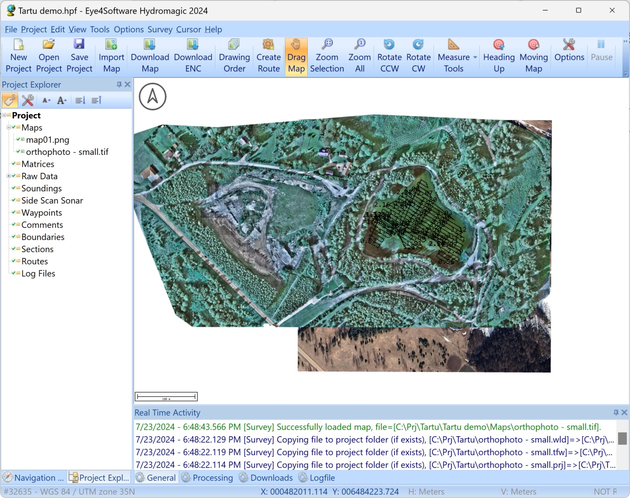
18. Zoom-in and check the numbers in raw data. This is "depth below transducer". Normally for bathymetric survey we need not the depth but bottom elevations - as depth is something volatile and we want to deliver more or less persistent results. We will generate elevations on the processing stage.
Initial processing
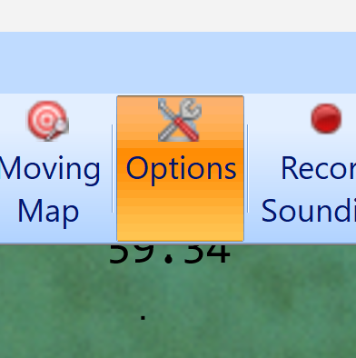
19. We have finished importing raw data and maps and can now begin processing the data. Here we need to do one preparatory step in the Hydromagic settings. Click Options in toolbar:

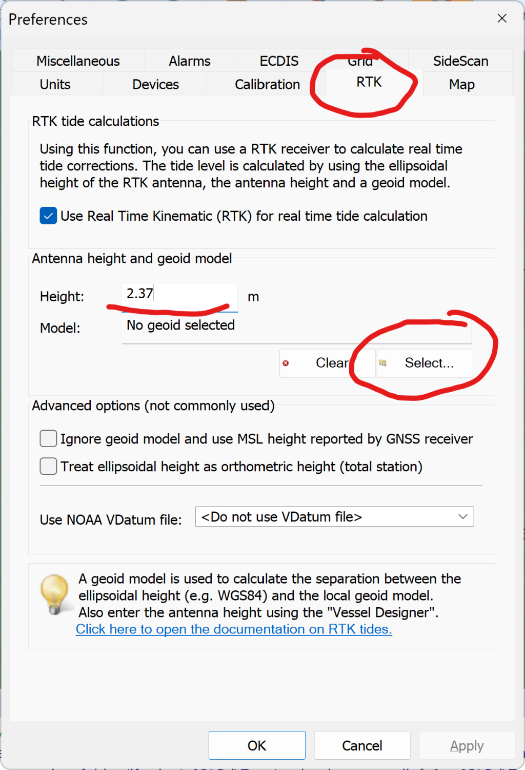
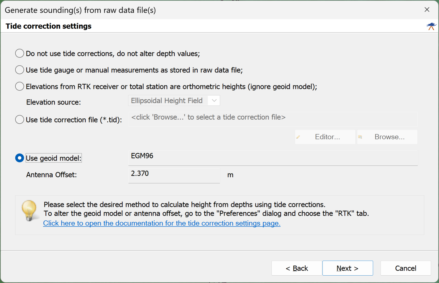
20. Select RTK tab, set "Use Real Time Kinematics..." checkbox, enter 2.37 as antenna height. This is the distance between base of RTK antenna of our system and the bottom of the echo sounder's transducer - the parameter, which should be measured on the system using measurement tape. Click Select to select geoid for our bottom elevation calculations.
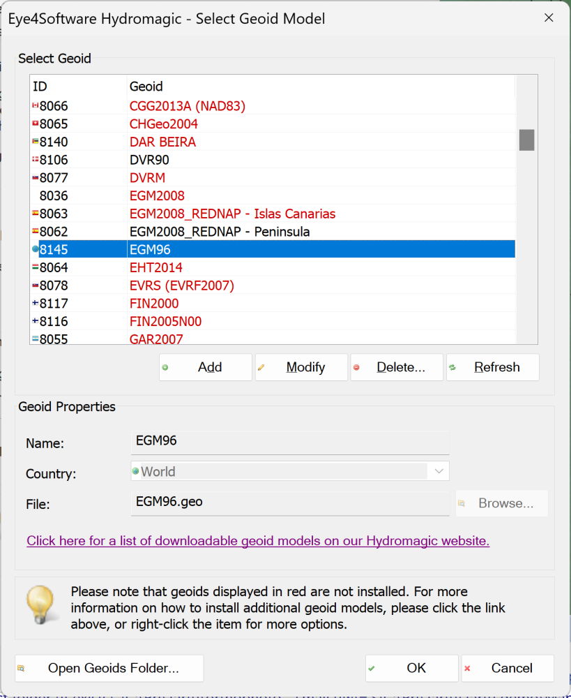
21. Here we need to select geoid. Unfortunately, Estonian latest official geoid file is license-protected, it is why you will not find it here in the list. You may find and request it for your own use, but in our "crash course" we will use global geoid. Find and select EGM96 and click OK two times to finish with settings.
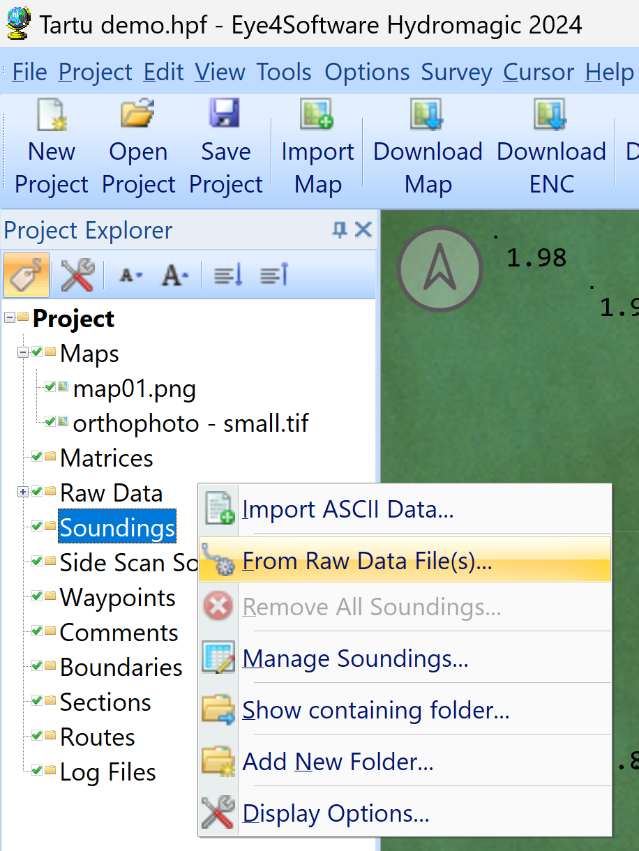
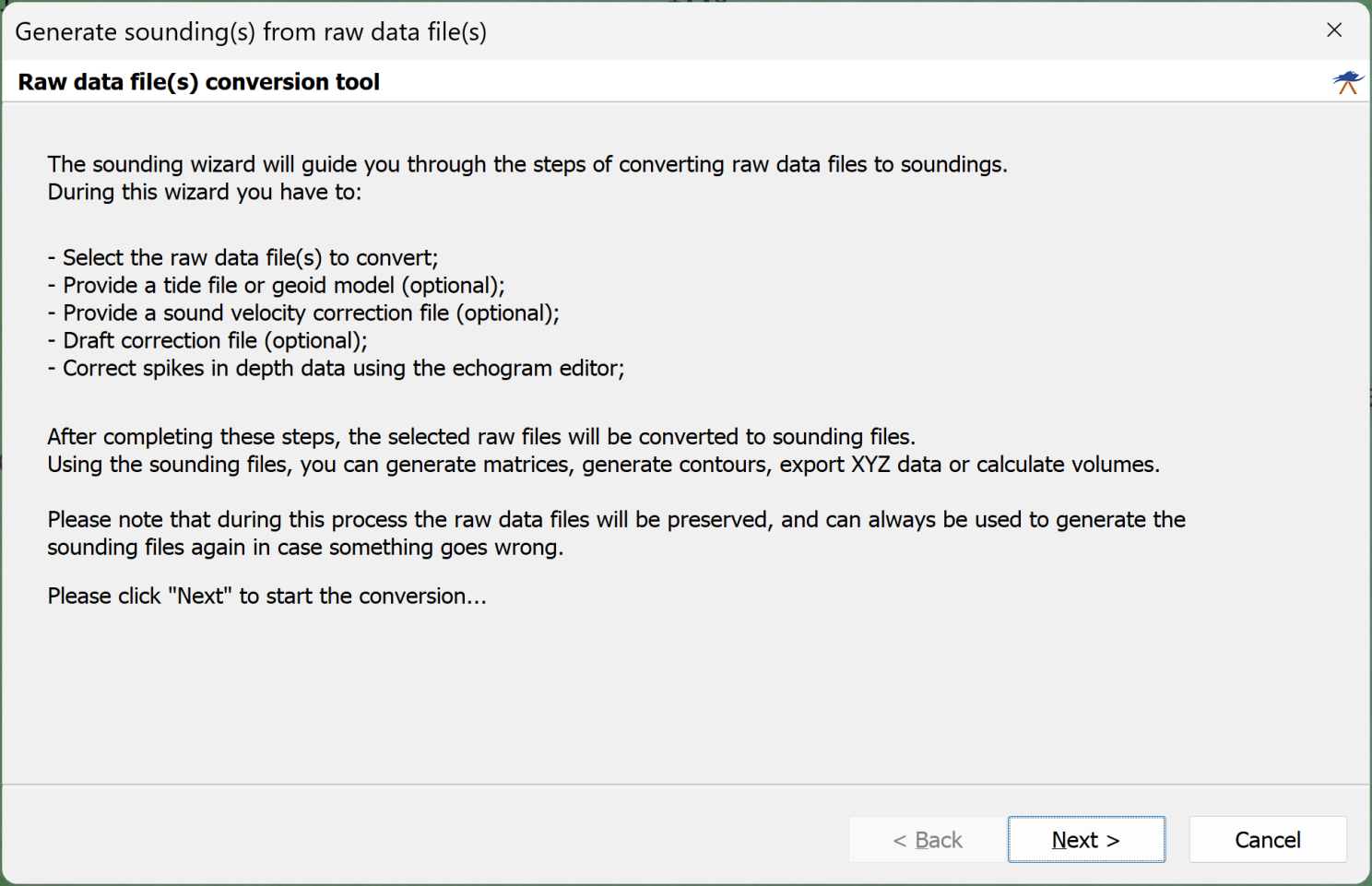
22. Right-click Soundings in Project Explorer and select "From Raw Data File(s)"
23. Click Next
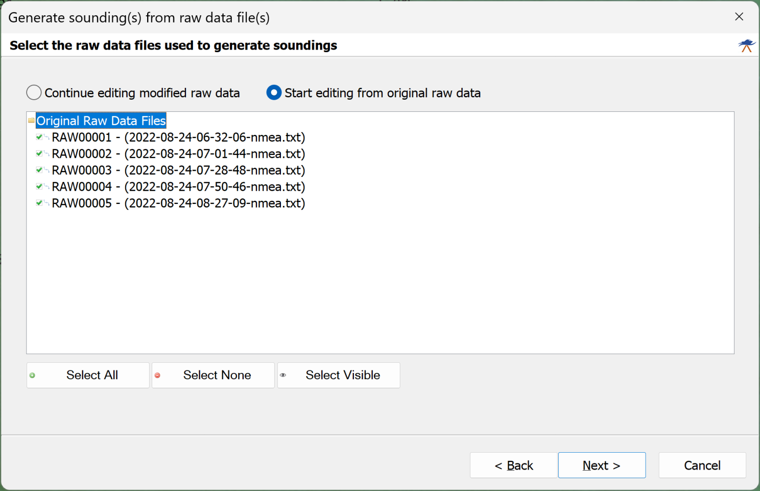
24. Select "Start editing from original raw data" and click "Select All". Click Next
25. Select "Use geoid model" and click Next
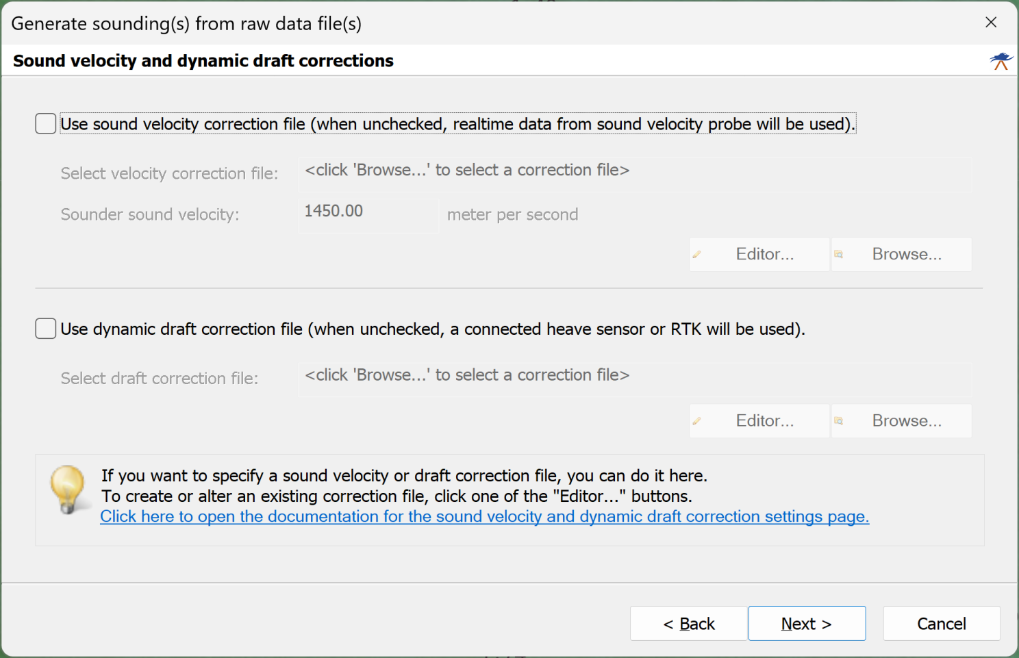
26. Click Next
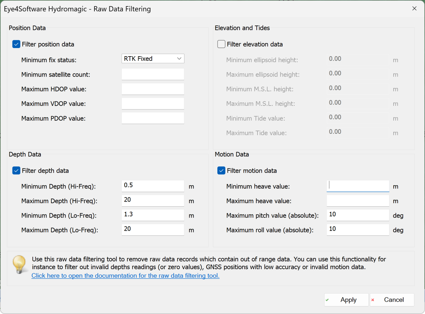
27. Click Filter
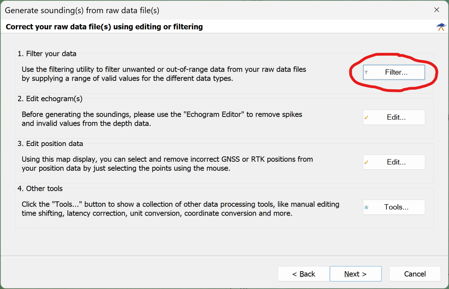
28. Select/fill fields as below and click Apply. These settings will filter-out all data values when position was recorded with low precision, or the depth was outside of expected/normal values, or echo sounder orientation was too far from vertical (Echologger ECT D052 echo sounder has internal pitch/roll sensors).
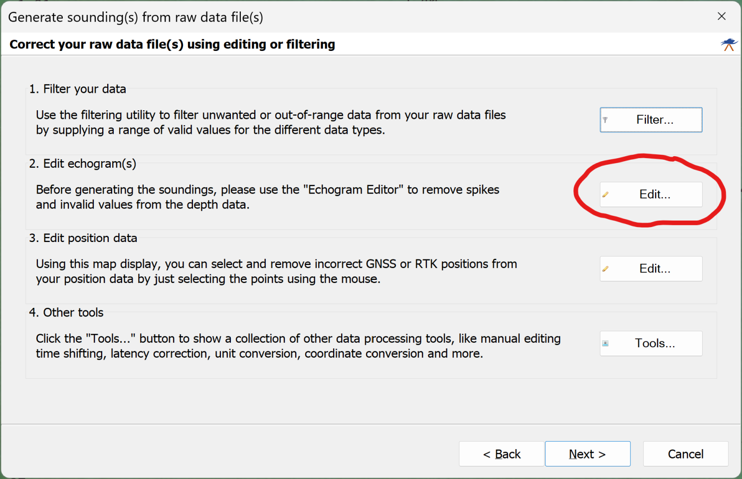
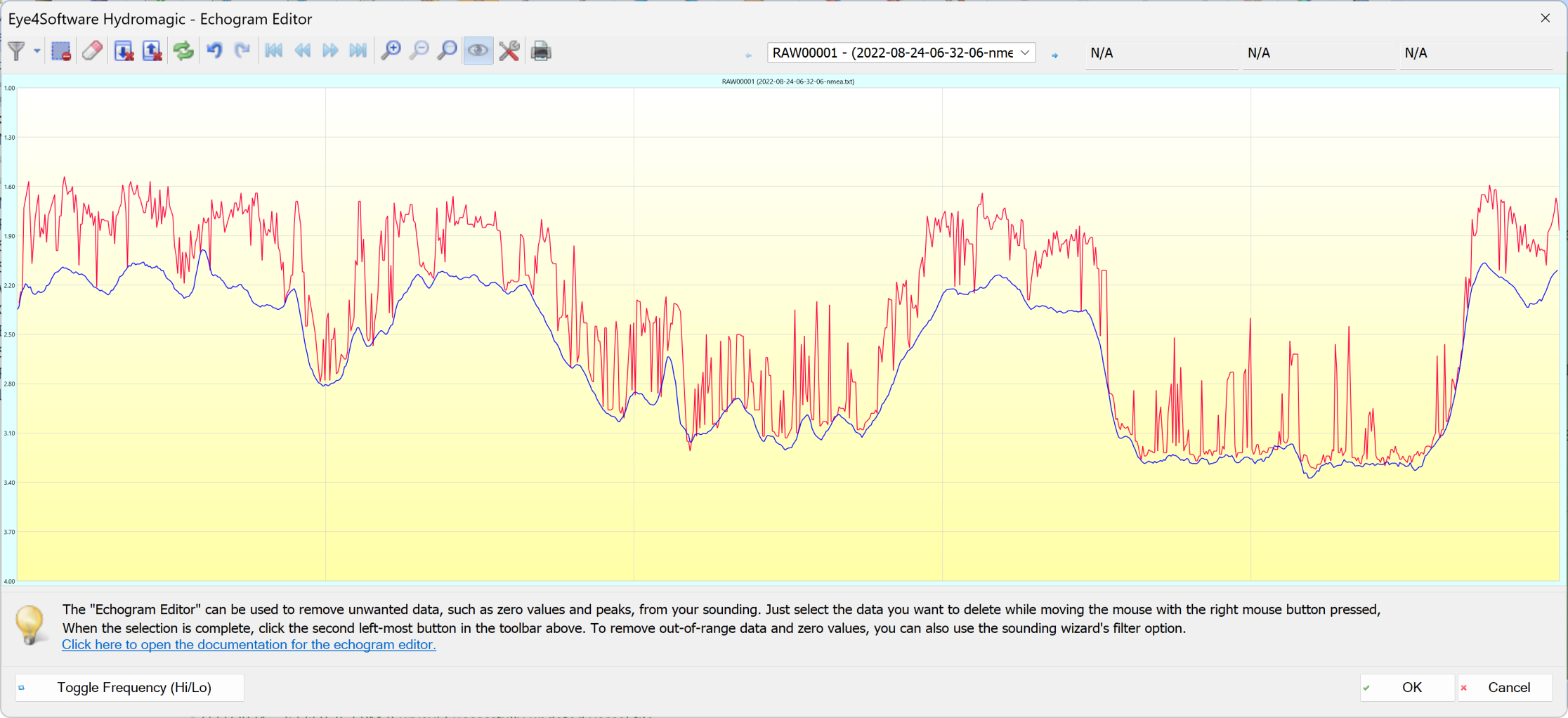
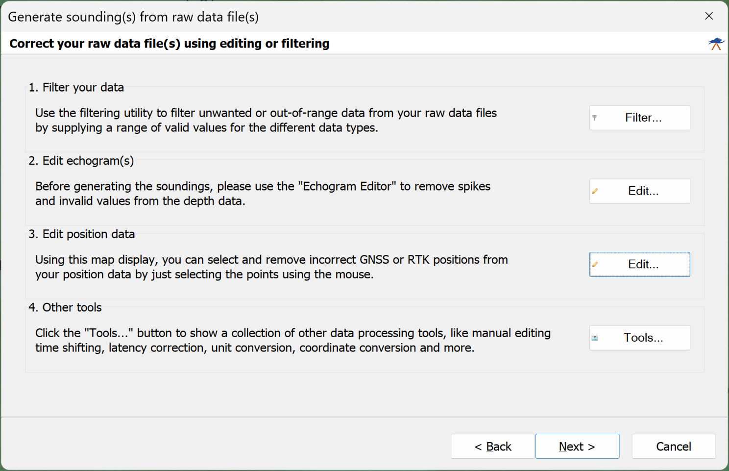
29. Click Edit
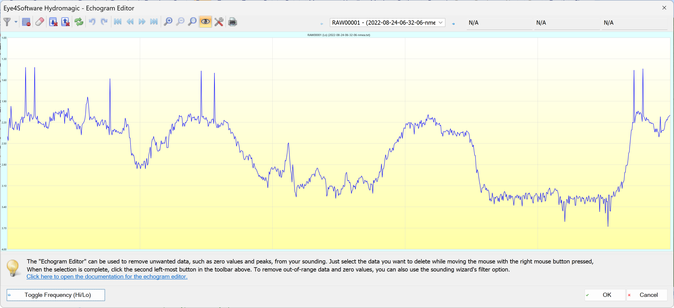
30. We will see something as on the screenshot below. If not - click few times button "Toggle Frequency (Hi/Lo)". Echo sounder ECT D052 is a dual-frequency device, so we may see two plots - for high and low frequencies. Low frequency (blue) plot here is a reflection from the lake's bottom, jumping red plot is reflection from seaweeds (vegetation) covering the bottom.
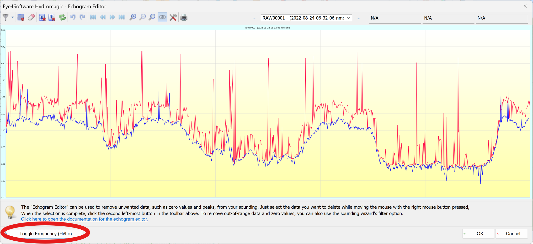
31. Now we need to clean the data a bit. Click "Toggle Frequency (Hi/Lo)" to see low-frequency measurements only.
32. Select obvious spikes by holding down the right mouse button
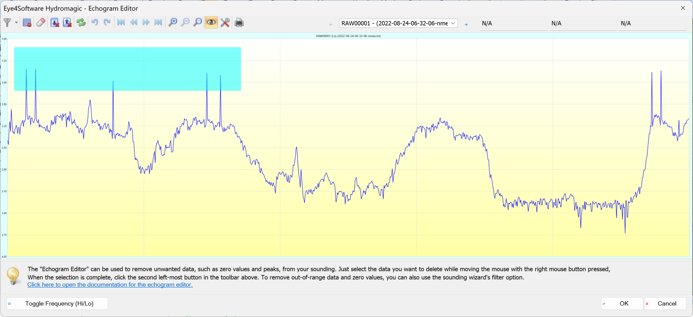
33. Click this icon or press Delete button on keyboard

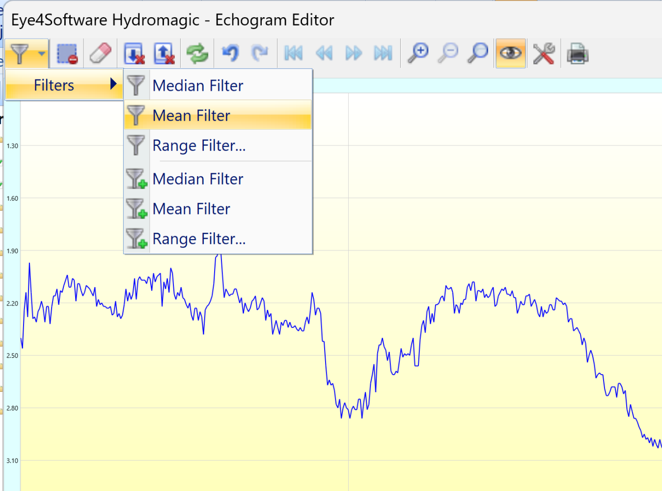
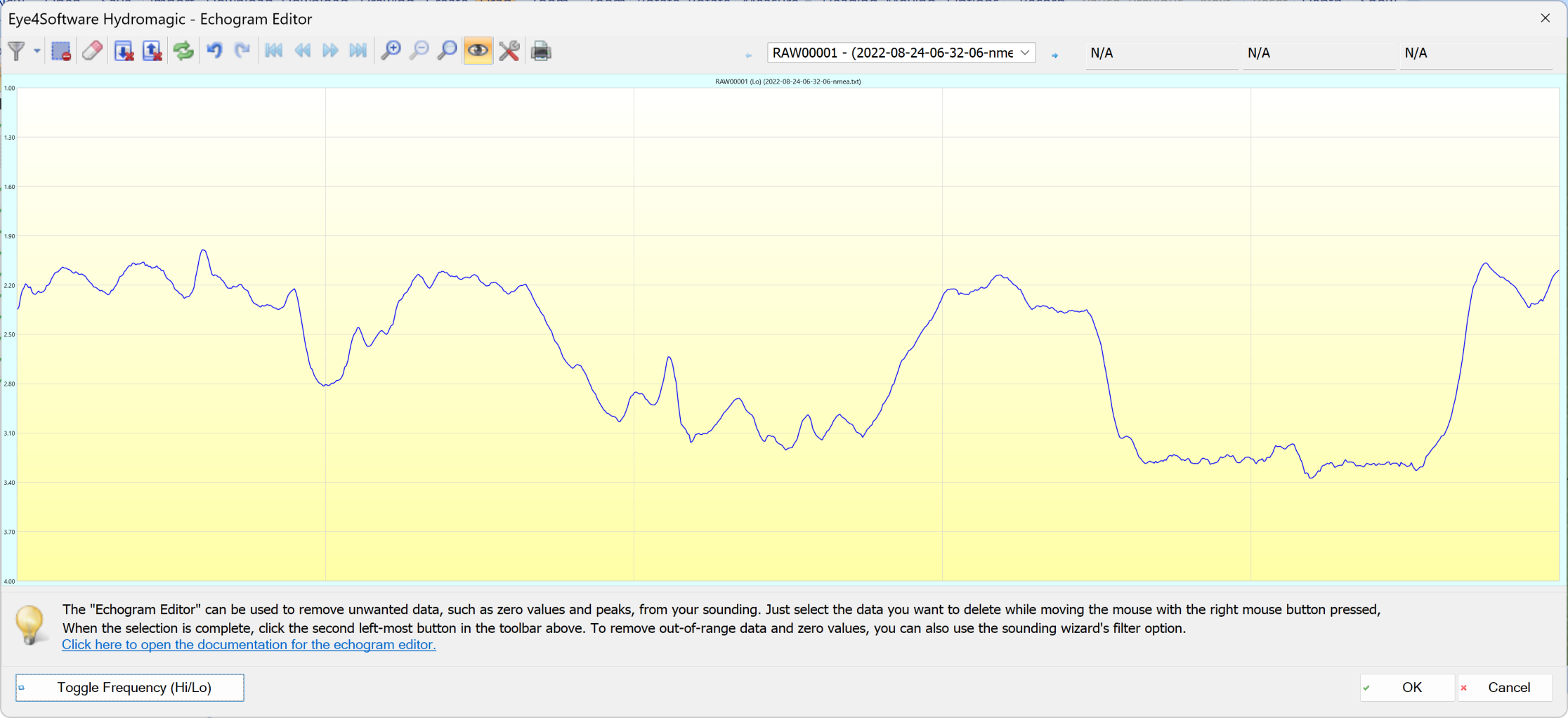
34. When you finish with manual cleaning, apply mean filter
The bottom profile will become much smoother:
35. Repeat cleaning for hi-frequency. Final result may look as below, but please don't spend too much time for the hi-frequency data in that and in similar cases - it's normal that hi-frequency readings are jumping up and down for the bottom covered with vegetation.
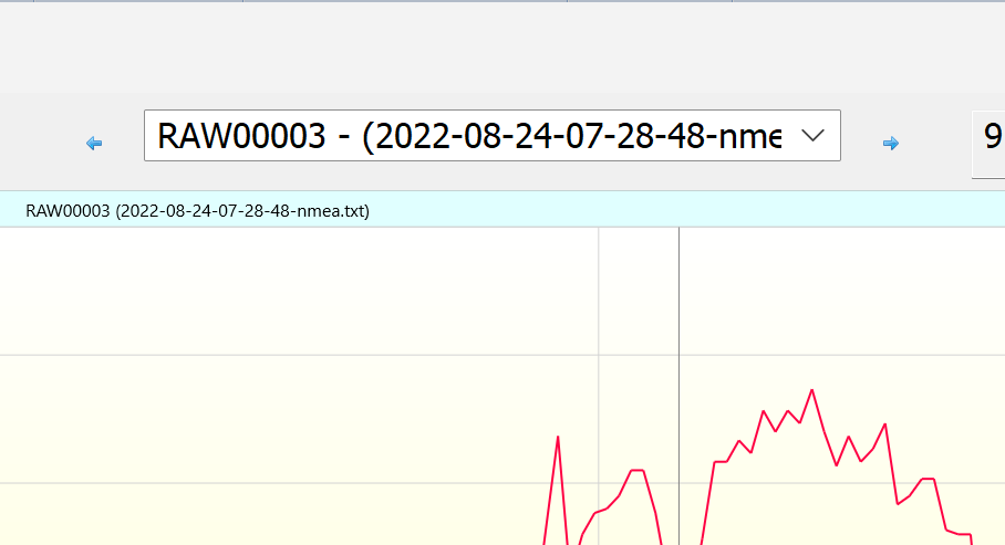
36. Repeat the same for all data files, use drop-down list or arrows to navigate between files. Click OK when you are satisfied.
37. You can also edit position data, but in many cases this step is optional. Click Next
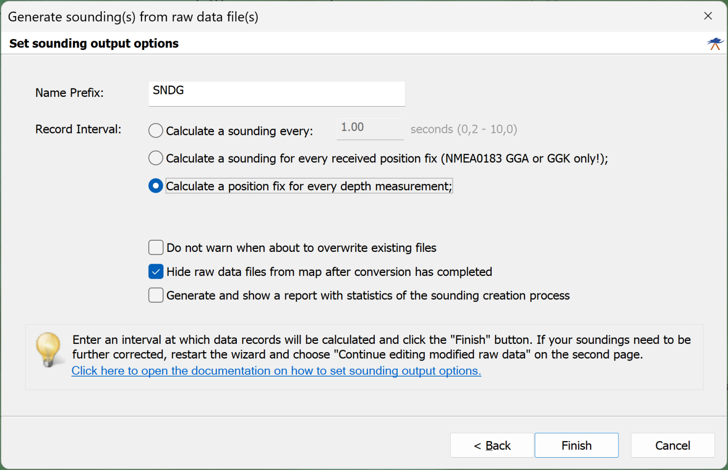
38. Click Finish
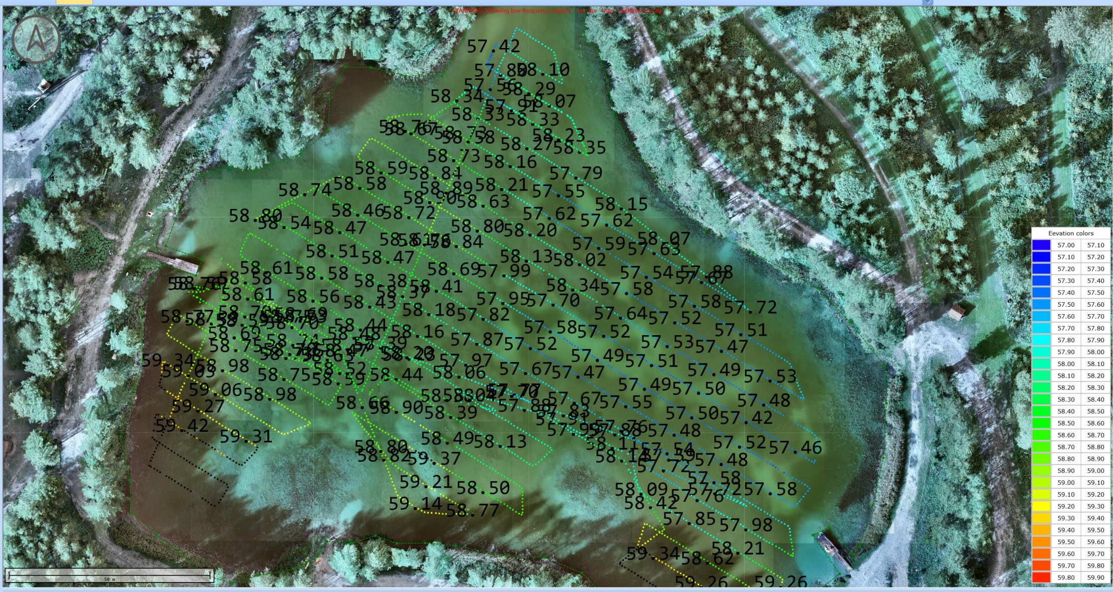
39. Zoom-in and check the numbers again. These numbers are bottom elevation in selected geoid, EGM96 in our case.
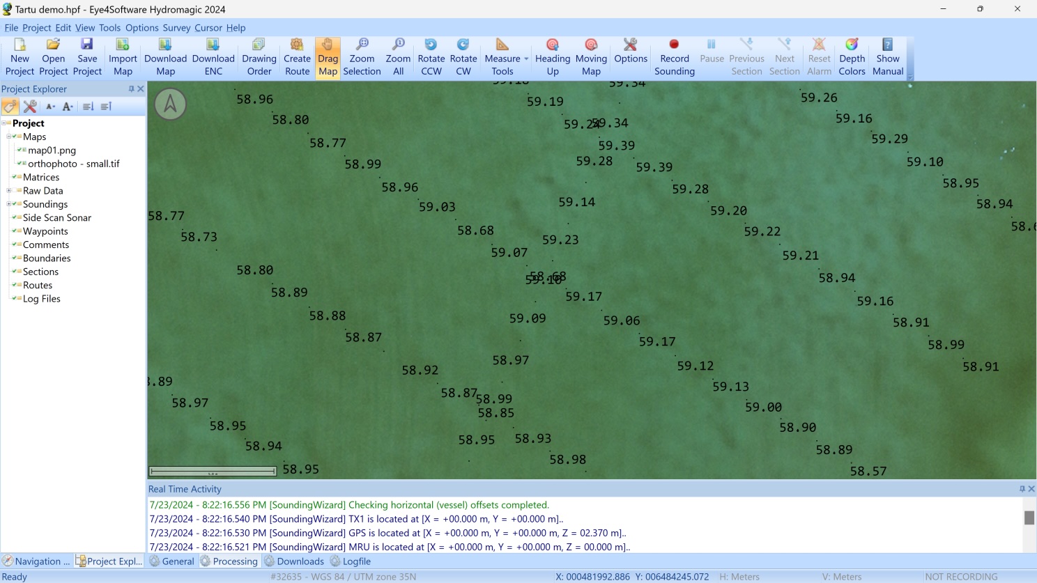
By default Hydromagic will display elevation based on high-frequency measurements. Remember that they are not robust in our case because of vegetation covering the bottom. So it's better to display values based on low-frequency.
40. Click Options
Select Map tab, set Show low frequency depths flag and click OK
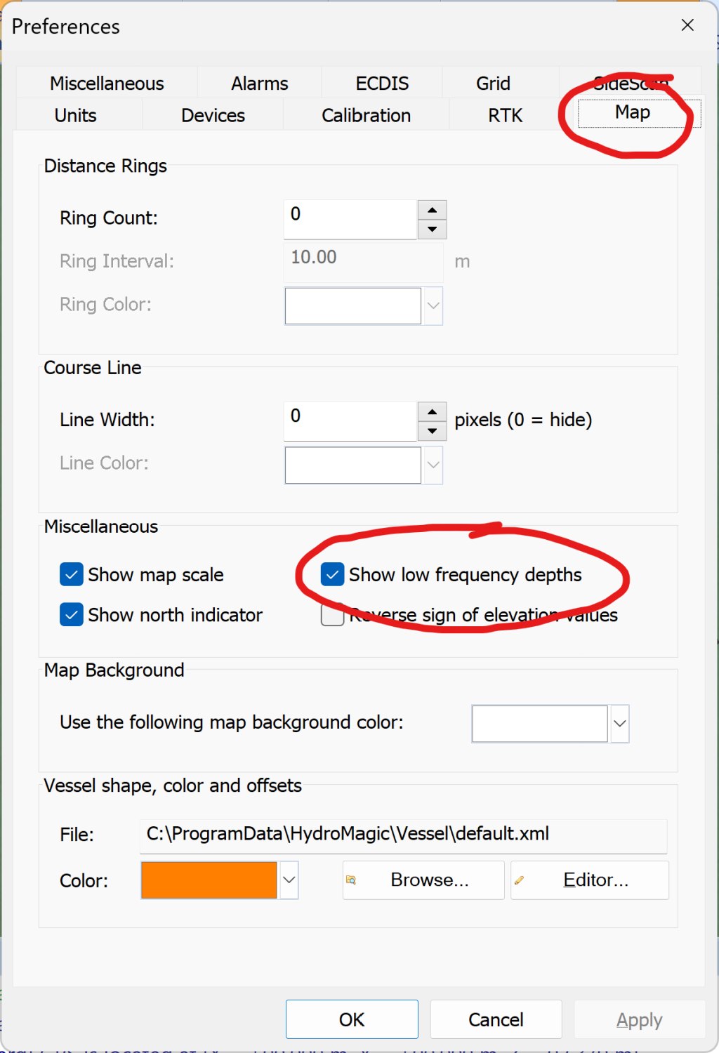
You may notice that the numbers have changed a bit.
Congratulations! We have processed the data.
Let's make our world colourful
Here we need to create color palette and use it to display our echo sounder data.
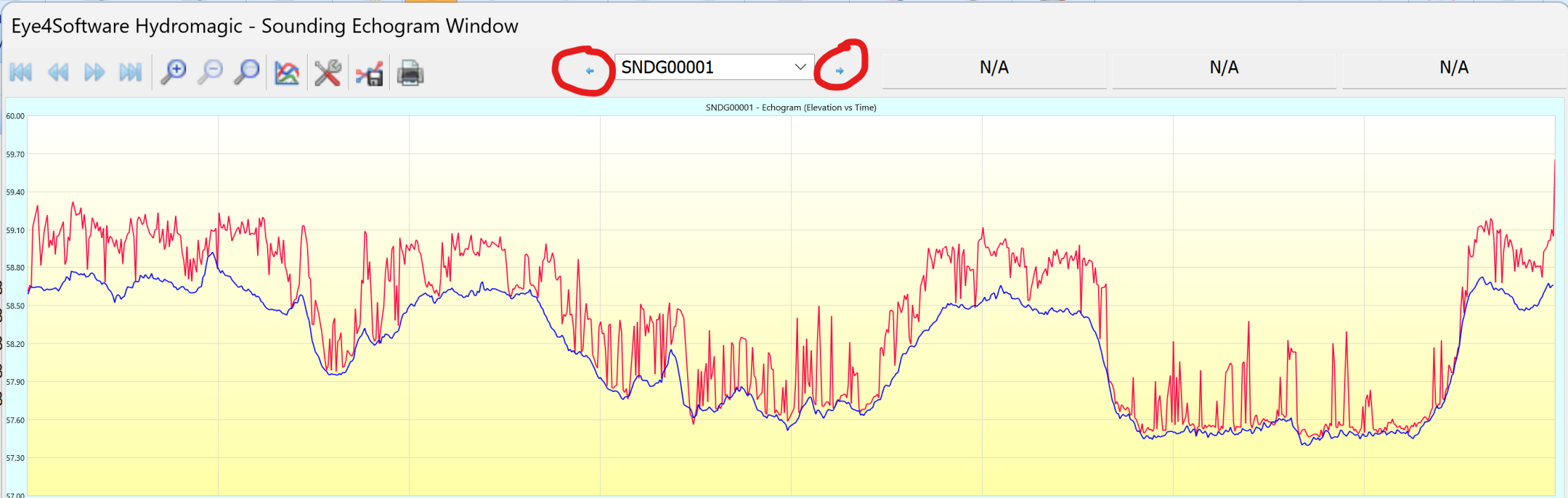
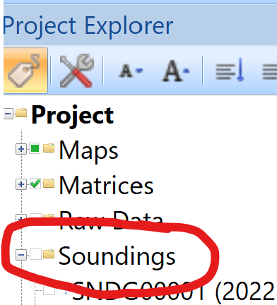
41. We need to know elevation range for our data set. Expand Soundings node in Project Explorer, right-click first sounding and select Show Echogram
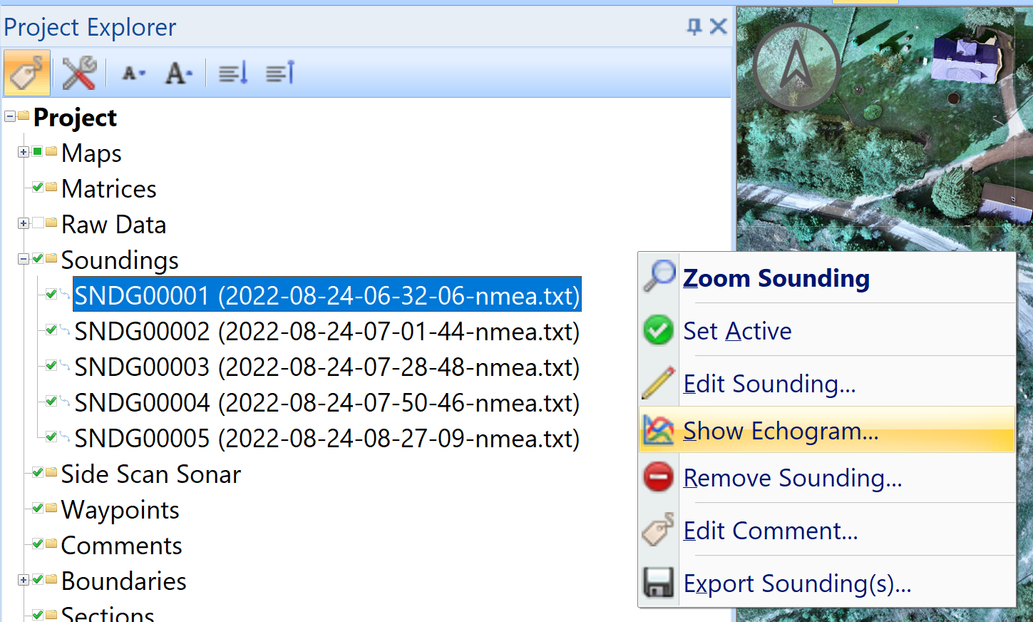
42. Scroll through sounding files and notice min/max elevation for low-frequency data (blue plot). All elevations are between 57 and 60m. Click Done to close the window.
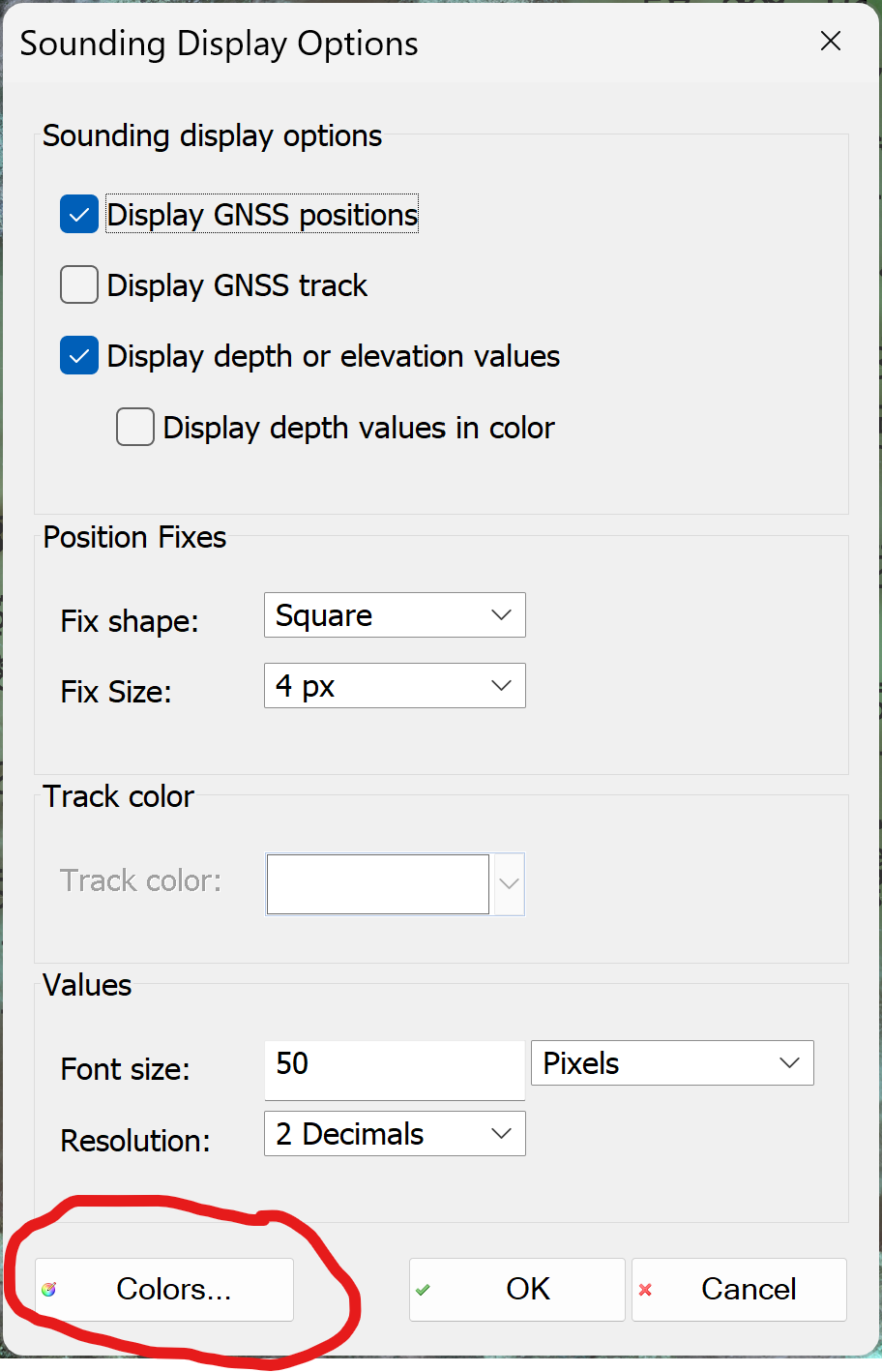
43. Right-click Soundings in Project Explorer and select Display Options

44. Click Colors
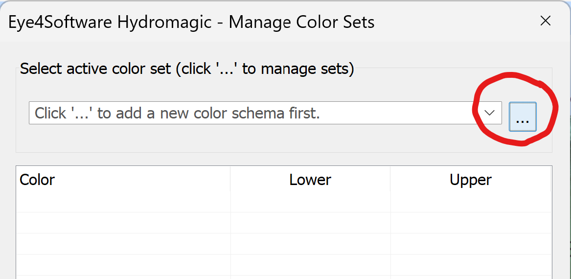
45. Click "..."
46. Click Add
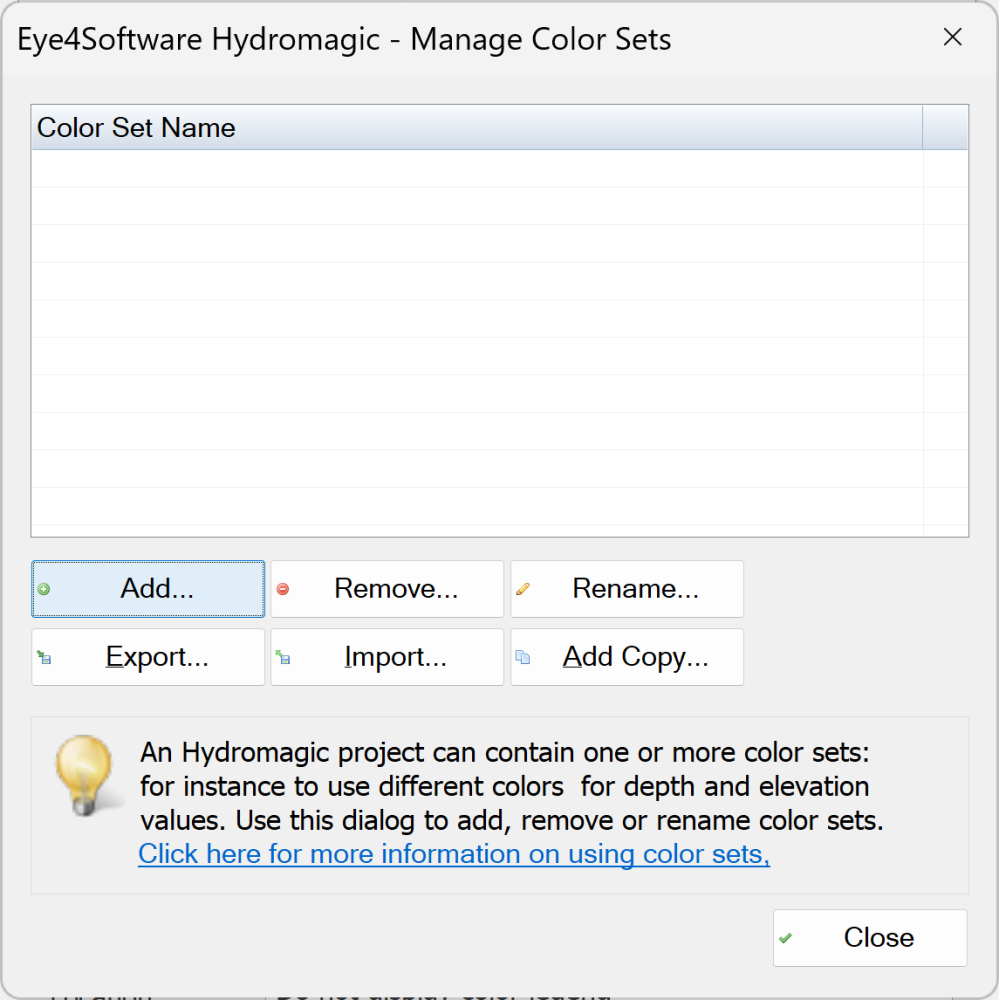
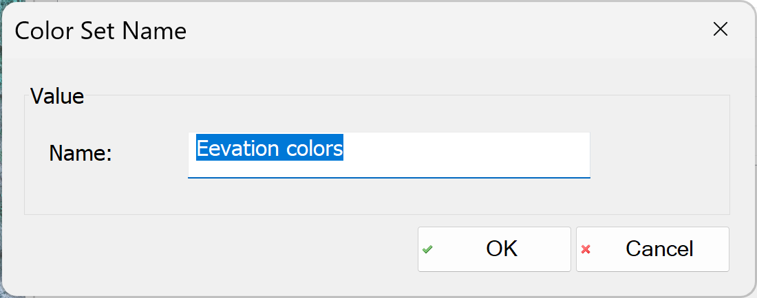
47. Enter the name for the color set (palette) and click OK and Close in previous window.
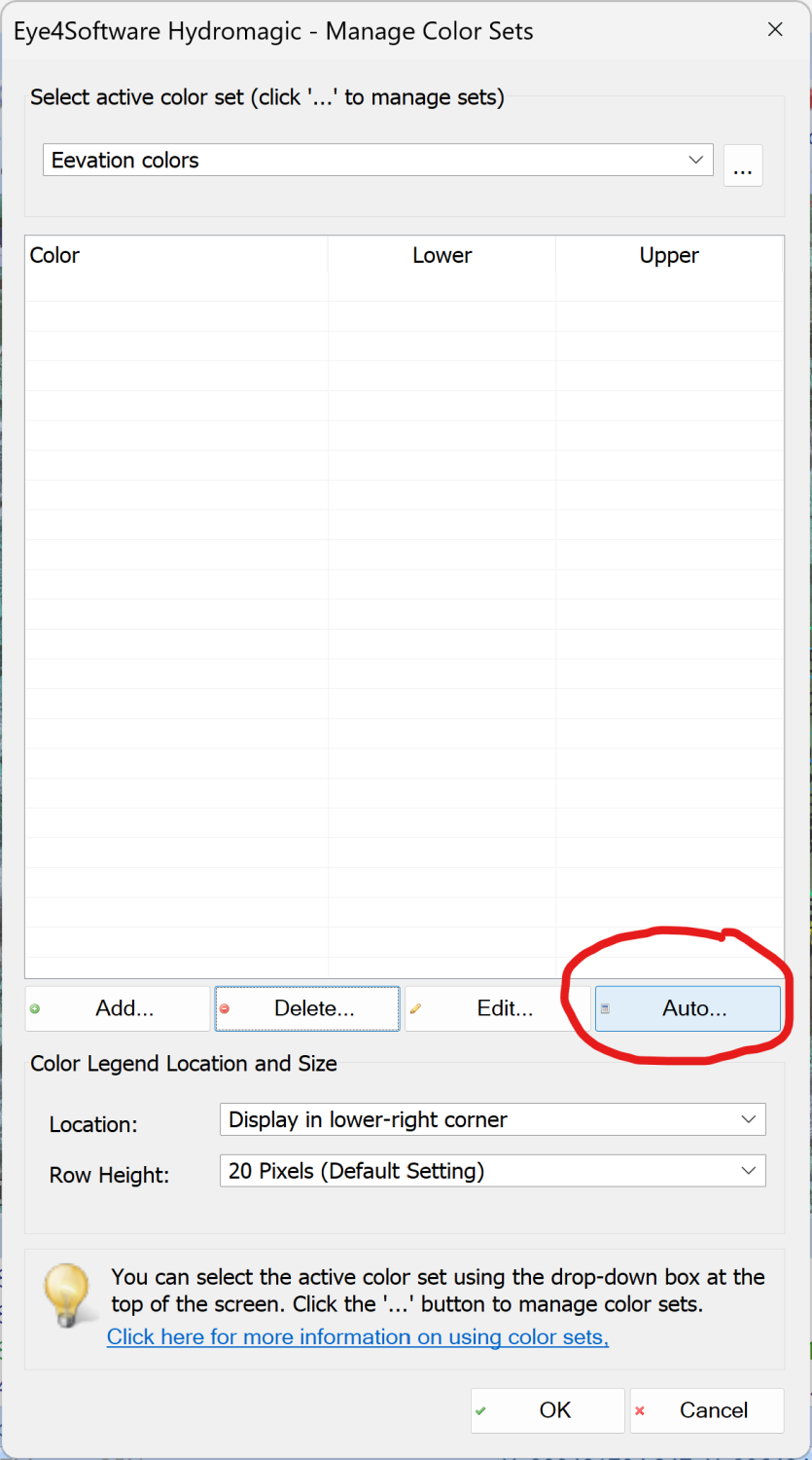
48. Click Auto
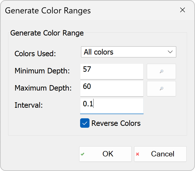
49. Enter the values as in the screenshot. 57 and 60 are the values we found earlier. Click OK.
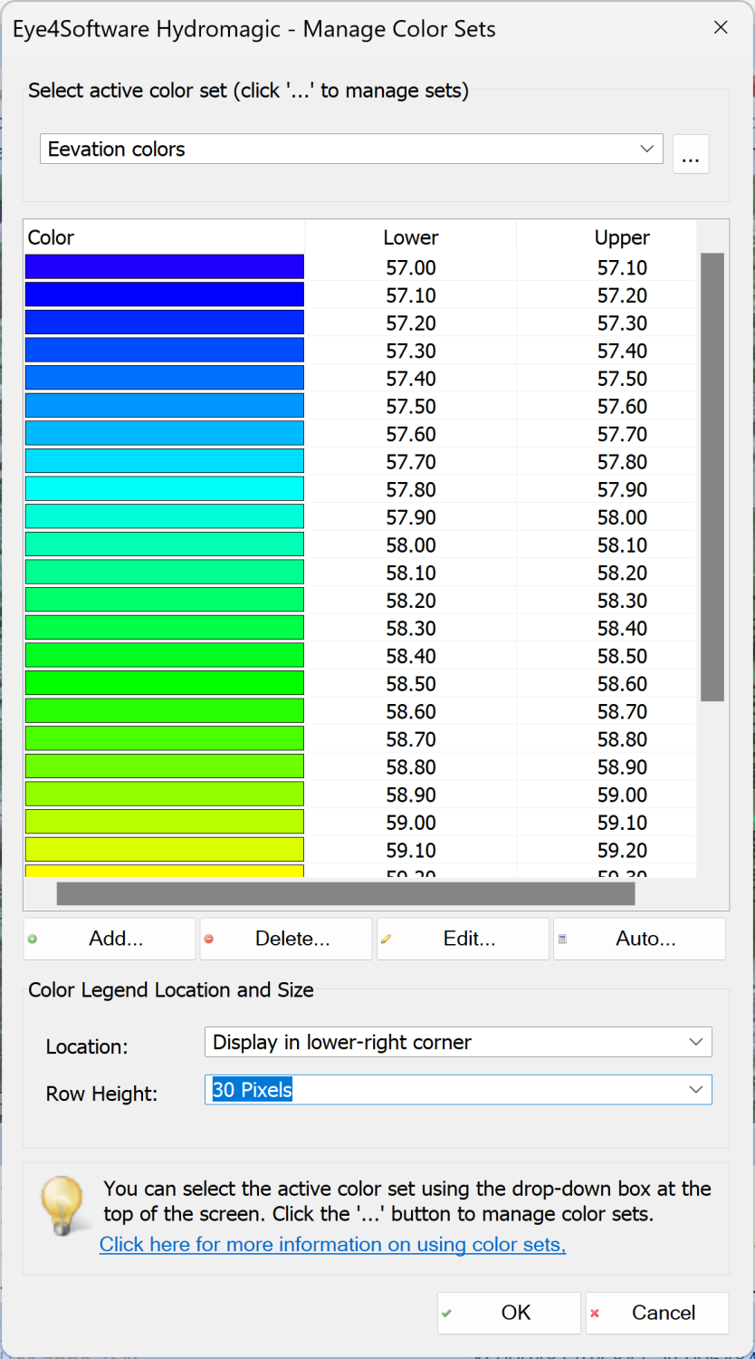
50. The color list will be filled with automatically generated values. Click OK in this window and again.
51. Now we can see that the measurement (sounding) points are displayed in color.
Matrix (elevation map) generation
Some bathymetric survey customers only require processed soundings as output. But quite often they order a elevation or depth matrix or a map.
Here we will generate the height matrix 2 times - without boundaries and using the lake boundary.
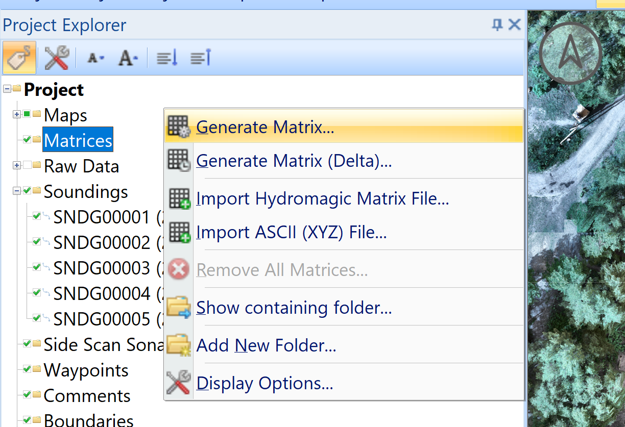
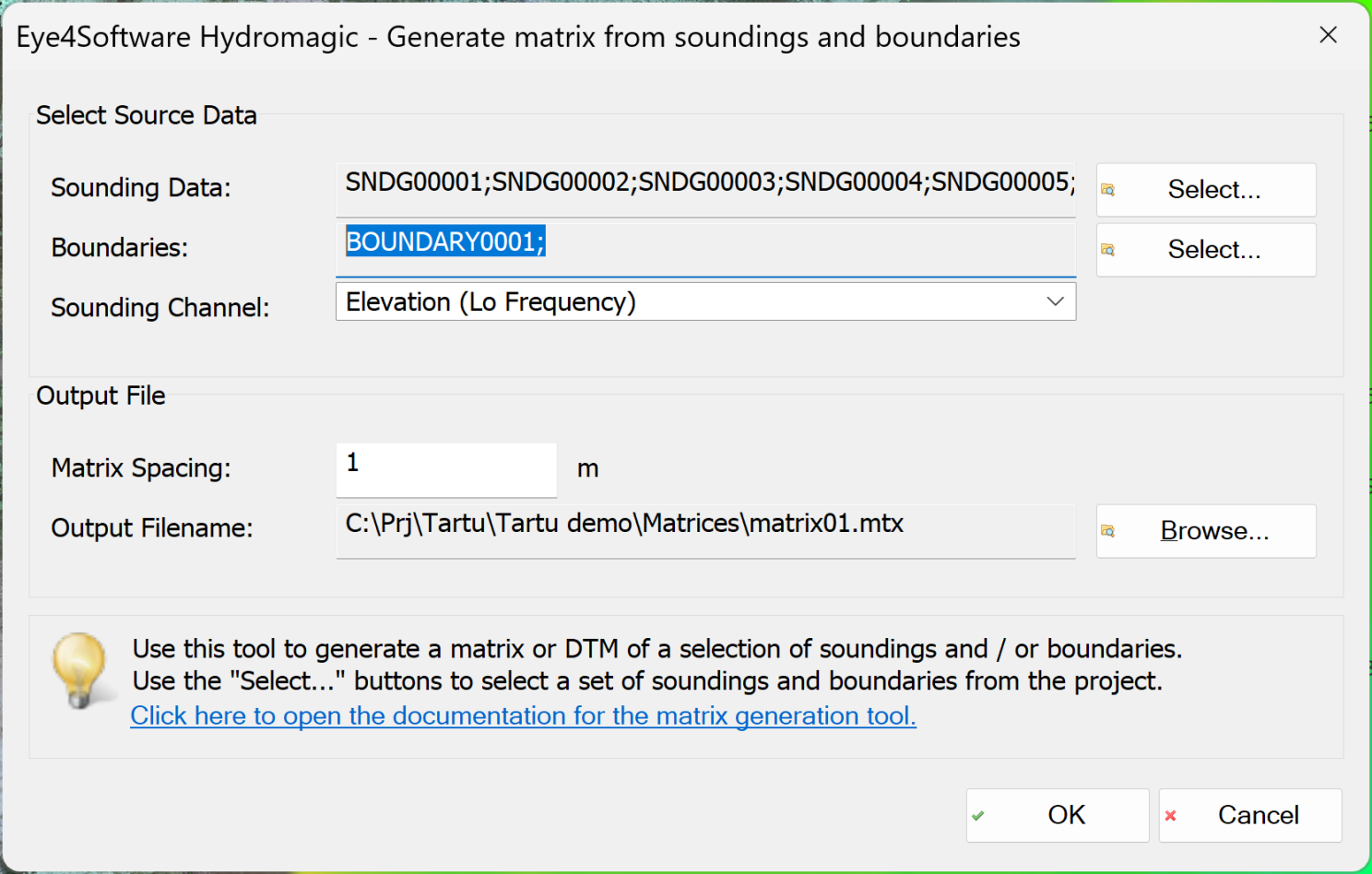
52. Right-click Matrices in Project Explorer and select Generate Matrix
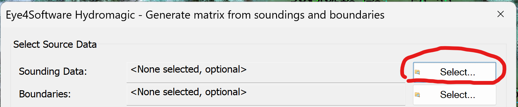
53. Click Select for Sounding Data
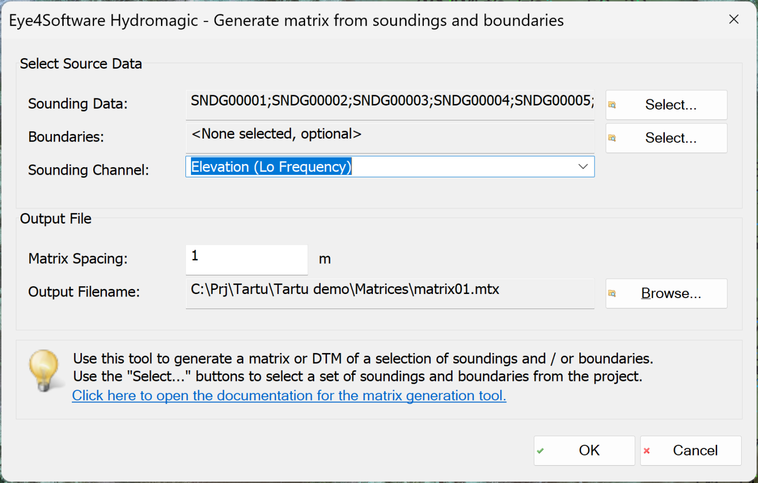
54. Click Select All and OK

55. Select Elevation (Lo Frequency) for Sounding Channel, 1m as Matrix Spacing and specify folder and filename for the matrix. Click OK.
56. Un-check Soundings node in Project Explorer
... and we will see an elevation map on top of the orthophoto:
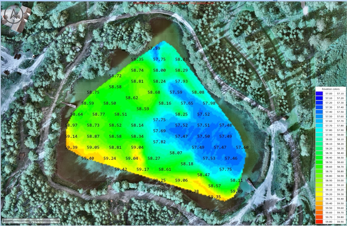
That matrix doesn't cover entire lake surface - because we don't have measurements close to the brink. We can extrapolate readings to cover entire water body with elevation map.
57. Right-click Boundaries in Project Explorer and select Draw Boundary

58. Using left mouse button draw boundary of lake using hi-resolution orthophoto map as background for digitizing. You can use mouse wheel for zoom-in/out. Right-click when you finish.
59. Boundary editor will appear on the screen. Check Include the elevation of this boundary in matrix generation and click Level.
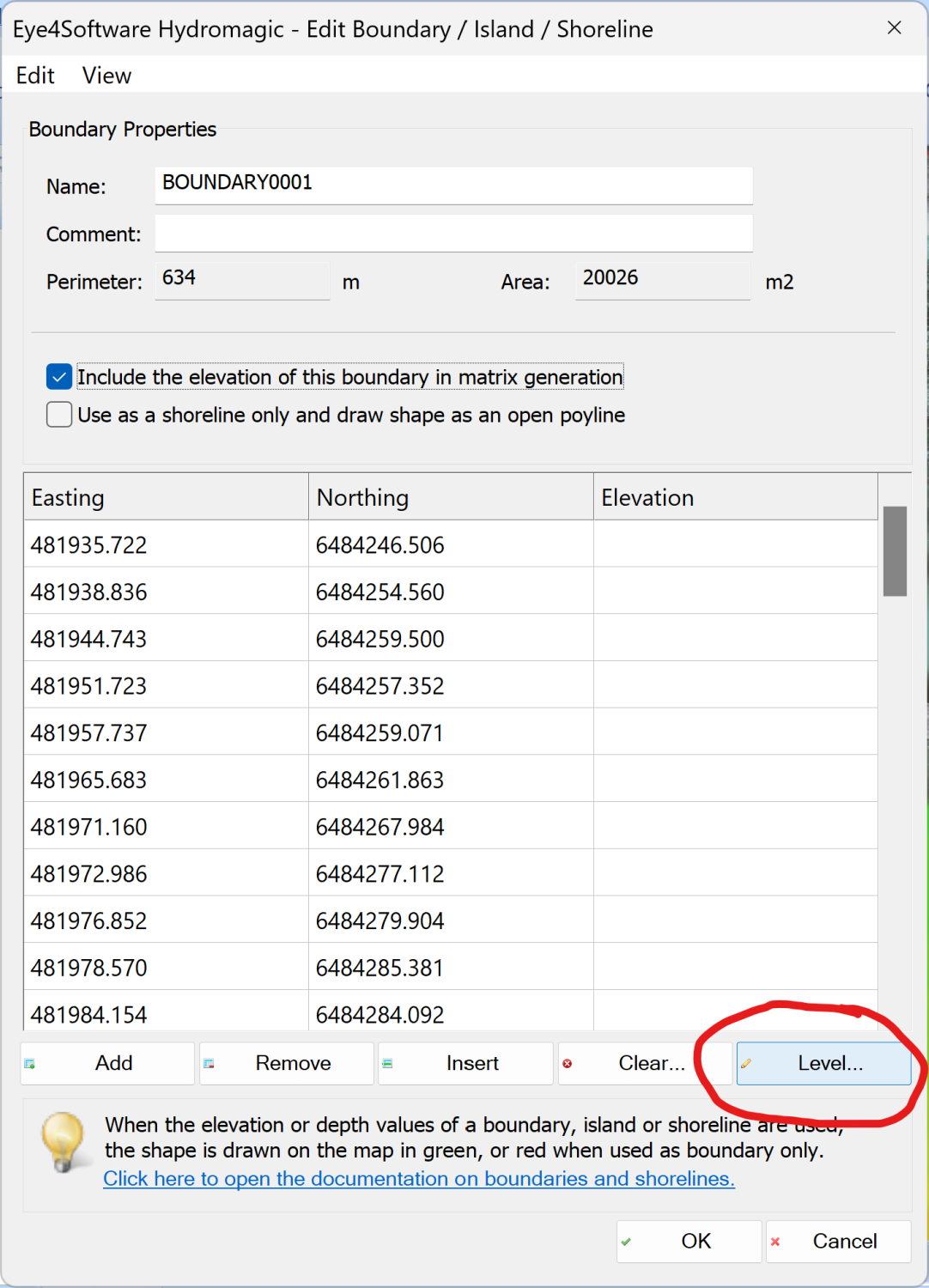
60. Enter 60 and click OK. This number is elevation of shoreline relative to the EGM96 geoid. I calculated this number using flight log data (using elevation of drone's RTK receiver and data from radar altimeter when drone was on survey lines over the water), but direct method is to use GNSS RTK/PPK receiver during data acquisition.
61. Notice that Elevation column is filled with 60s, and click OK.
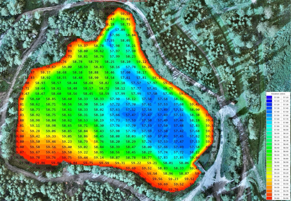
62. Repeat the matrix generation, but select boundary this time
63. Now elevation map covers entire lake:
What next?
We have completed all the standard steps for processing bathymetric data, and you can see that it is not rocket science at all.
The next standard steps are:
- Quality control using control lines or survey line intersections;
- Create and export output files and reports.
Both topics are also not complex, but they will be covered in separate articles or in one of my webinars. Stay tuned!


.jpg)
